Happy New Year!
This post presents a script implementation of CreditMetrics VaR calculation in python. The code follows the calculations and standards in R ‘CreditMetrics’ Package from CRAN.
CreditMetrics was developed by J.P Morgan in 1997 and is used as a tool for accessing portfolio risk due to changes in debt value caused by changes in credit quality.
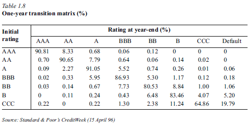
It takes a Migration Matrix (usually provided by a credit rating agency)
- The Migration Matrix uses historical transition probabilities between rating classes
To compute the loss distribution, the tool needs the following information
- Probability of Default (PD): risk of losing money
- Exposure At Default (EAD): amount of risk
- Recovery Rate (RR): the fraction of EAD that may be recovered when default happens
- Credit Spread: used to calculate expected market value for securities with different ratings
With simulation we can also get a distribution of loss
- Idea: company return V are assumed to be standard normal distributed V ~ N(0,1) and simulated
- Company value V at time t determines the rating at time t
- Migration thresholds can be computed from the transition probabilities
- Taking a BB rated issuer from the migration Matrix, we can build a standard normal density function and the thresholds (cut-off) of each rating using normal inverse function
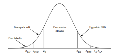
- Migration Thresholds have to be computed for each output ratings
- e.g. Default threshold is the quintile for the probability of default
- ZD = N-1(PD) , N-1 is the inverse function of the standard normal distribution and PD is the probability of default (given by the Migration Matrix)
- Threshold for migration to CCC is
- ZCCC = N-1(PD + Pccc)
- Credit Spread is the risk premium demanded by the market
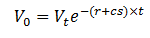
- Under risk neutral probabilities
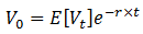
- And if Default happens, the expected value of V is

- Rearrange the above equation we get
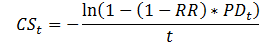
- t = 1 for one year migration matrix
To simulate correlated random variables, use Cholesky Decomposition
(Note, this is a simplified approach of CreditMetrics and it’s assuming a constant default correlation, in practice this can be estimated using asset correlations; the VaR calculated from this framework does not capture market risk – interest rate movement)
Example:
Assume, there are 3 assets with exposure of [1590899,1007000,188000] in the portfolio
Total exposure:2,785,899
Their ratings are [BBB, AA, B]; In code we use their indices in the transition matrix.
Recover rate = 55%
1% CreditVaR = 140,388.88
1% Shortfall = 310,713.24
 from __future__ import division
import pandas as pd
import numpy as np
from scipy.stats import norm

from numpy.linalg import cholesky

# User inputs
TransMat = np.matrix("""
90.81, 8.33, 0.68, 0.06, 0.08, 0.02, 0.01, 0.01;
0.70, 90.65, 7.79, 0.64, 0.06, 0.13, 0.02, 0.01;
0.09, 2.27, 91.05, 5.52, 0.74, 0.26, 0.01, 0.06;
0.02, 0.33, 5.95, 85.93, 5.30, 1.17, 1.12, 0.18;
0.03, 0.14, 0.67, 7.73, 80.53, 8.84, 1.00, 1.06;
0.01, 0.11, 0.24, 0.43, 6.48, 83.46, 4.07, 5.20;
0.21, 0, 0.22, 1.30, 2.38, 11.24, 64.86, 19.79""")/100

N = 3 # number of asset
Nsim = 5000 # num sim for CVaR
r = 0 # risk free rate
exposure = np.matrix([1590899,1007000,188000]).T
recover = 0.55
LGD = 1- recover
idx = [3, 1, 5] # rating index start at 0
t= 1

# correlation matrix
rho = 0.4
sigma = rho*np.ones((N,N))
sigma = sigma -np.diag(np.diag(sigma)) + np.eye(N)

# compute the cut off for each credit rating
Z=np.cumsum(np.flipud(TransMat.T),0)
Z[Z>=1] = 1-1/1e12;
Z[Z<=0] = 0+1/1e12;

CutOffs=norm.ppf(Z,0,1) # compute cut offes by inverting normal distribution

# credit spread implied by transmat
PD_t = TransMat[:,-1] # default probability at t
credit_spread = -np.log(1-LGD*PD_t)/1

# simulate jointly normals with sigma as vcov matrix
# use cholesky decomposition

c = cholesky(sigma)
# cut off matrix for each bond based on their ratings
cut = np.matrix(CutOffs[:,idx]).T
# reference value
EV = np.multiply(exposure, np.exp(-(r+credit_spread[idx])*t))
PORT_V = sum(EV)

# bond state variable for security Value
cp = np.tile(credit_spread.T,[N,1])
state = np.multiply(exposure,np.exp(-(r+cp)*t))
state = np.append(state,np.multiply(exposure,recover),axis=1) #last column is default case
states = np.fliplr(state) # keep in same order as credit cutoff

Loss=np.zeros((N,Nsim)) # initialization of value array for MC

# Monte Carlo Simulation Nsim times
for i in range(0,Nsim):
    YY = np.matrix(np.random.normal(size=3))
    rr = c*YY.T
    rating = rr<cut
    rate_idx = rating.shape[1]-np.sum(rating,1) # index of the rating
    row_idx = xrange(0,N)
    col_idx = np.squeeze(np.asarray(rate_idx))
    V_t = states[row_idx,col_idx] # retrieve the corresponding state value of the exposure
    Loss_t = V_t-EV.T
    Loss[:,i] = Loss_t

Portfolio_MC_Loss = np.sum(Loss,0)
Port_Var = -1*np.percentile(Portfolio_MC_Loss,1)
ES = -1*np.mean(Portfolio_MC_Loss[Portfolio_MC_Loss<-1*Port_Var])
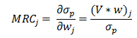
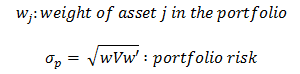
 be a vector of all asset weights
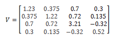
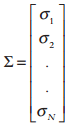 be a vector of all asset volatility (square root of the diagnal of V, the covariance matrix)
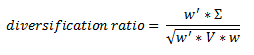
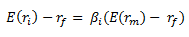
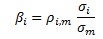
 is not a constant because correlation of stock return to market return varies across assets/stocks. But Beta is indeed positively correlated with asset volatility, thus the expected excess return is positively correlated with asset volatility under the CAPM.

 Then
Then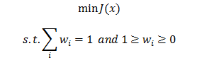 In python
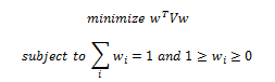
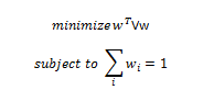
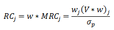
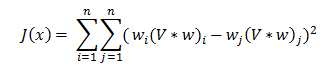
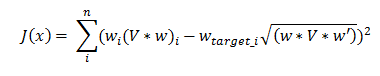 you can set up your target risk allocation for each asset then minimise the objective function of squared error
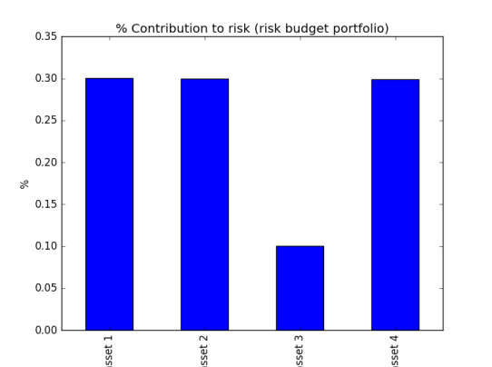
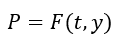
 we define
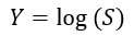
 Then
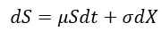
Then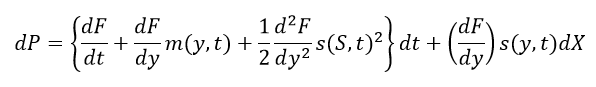 Then we plug the following variables into the Ito’s Lemma
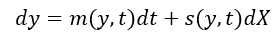
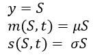 After rearrangements, and substituting the PDE of Y=log(S) with respect to S and t, we get
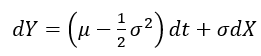 and
and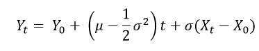 Since
Since